PowerShell into Excel - ImportExcel Module Part 2

Last week I have introduced you to ImportExcel PowerShell module and its capability to manipulate the worksheets and create pivot tables and pivot charts. This week let’s jump on some other features: conditional formatting and charts.

ImportExcel – how to?

If you have not installed the module before, use the below code to do so and move on to the examples.

# get the module
Set-ExecutionPolicy Bypass -Scope Process
Install-Module -Name ImportExcel
Import-Module -Name ImportExcel

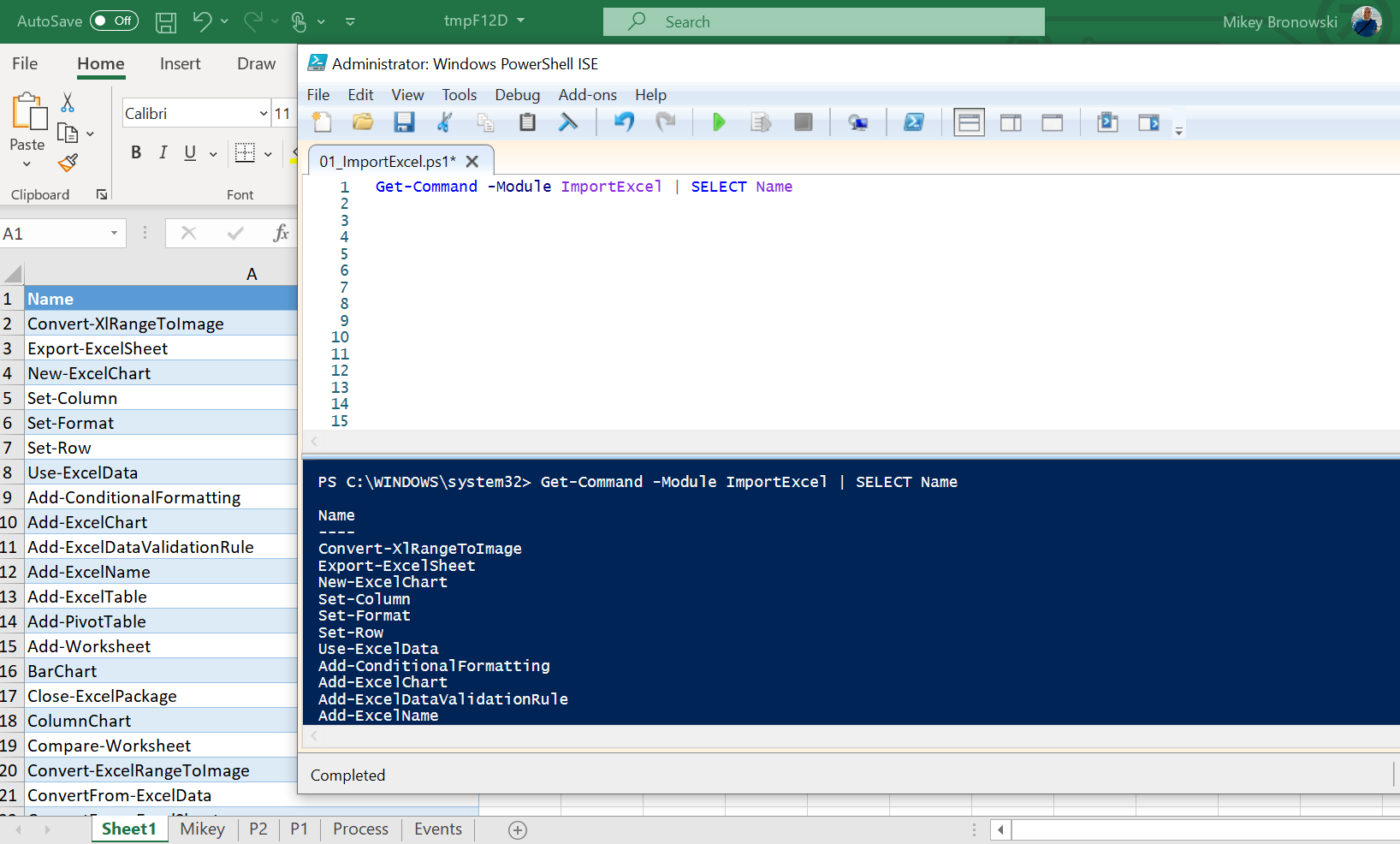
ImportExcel – how to do conditional formatting?

I have a dataset with three columns and would like to add the conditional formatting on each of the columns separately. As a base will use Events exported to the worksheet and later will use the Export-Excel function with ConditionalFormat parameter:

# cleanup any previous files
$excelFile = "$env:TEMP\MikeyEvents.xlsx"
Remove-Item $excelFile -ErrorAction SilentlyContinue
# create a new file in TEMP location - clean worksheet
$events = Get-EventLog -After (Get-Date -Format 'yyyy-MM-dd') -LogName system | SELECT EventID, Category, EntryType
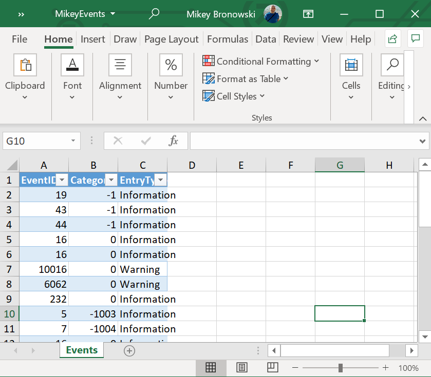
$events | Export-Excel -WorksheetName Events -TableName Events -Path $excelFile -KillExcel

That will produce spreadsheet like this:

Now, will add another worksheet with the Conditional Formatting:

# define conditional formatting for each column in a new worksheet
# these are random formats, just to show the capability
$ConditionalFormat =$(
    New-ConditionalText -ConditionalType AboveAverage -Range 'A:A' -BackgroundColor Red -ConditionalTextColor Black
    New-ConditionalText -ConditionalType DuplicateValues -Range 'B:B' -BackgroundColor Orange -ConditionalTextColor Black
    New-ConditionalText -Text Information -Range 'C:C' -BackgroundColor Blue -ConditionalTextColor Yellow
)
# add the new worksheet with ConditionalFormat.
$Events | Export-Excel -WorksheetName EventsConditional -TableName EventsConditional -Path $excelFile -ConditionalFormat $ConditionalFormat -Show -Activate -KillExcel

That is how to the other worksheet looks like one below:

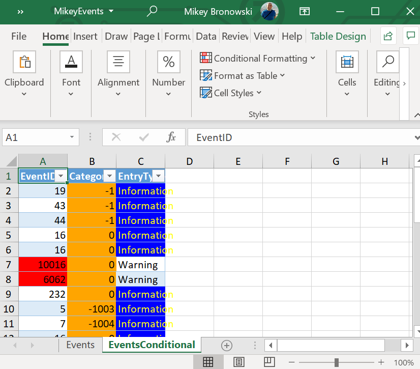
We have gotten some colors. It is also possible to apply the formatting to the existing worksheet. For that scenario I will define the formatting first (keeping in mind I will place the second table on the side of existing one).

# prepare formatting for the second table on the same worksheet - shifted two columns to the right 
# columns A,B,C will become E,F,G
$ConditionalFormat2 =$(
    New-ConditionalText -conditionalType AboveAverage -Range 'E:E' -BackgroundColor Red -ConditionalTextColor Black 
    New-ConditionalText -conditionalType DuplicateValues -Range 'F:F' -BackgroundColor Orange -ConditionalTextColor Black
    New-ConditionalText -Text 'Information' -Range 'G:G' -BackgroundColor Blue -ConditionalTextColor Yellow
)
# now to create the new table in the existing worksheet
# note the -StartColumn switch
$Events | Export-Excel -WorksheetName Events -TableName EventsConditional2 -Path $excelFile -ConditionalFormat $ConditionalFormat2 -Show -Activate -KillExcel -StartColumn 5

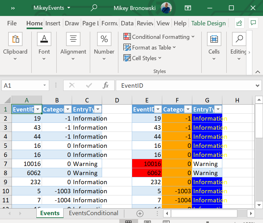
We are back on the first worksheet with to tables (first without, second with the conditional formatting applied).

On a separate note we can add conditional formatting using dedicated function called Add-ConditionalFormatting.

# load the spreadsheet
$excel = Open-ExcelPackage -Path $excelFile -KillExcel
# add new formatting for column G (second table)
# note how I am referring the worksheet
Add-ConditionalFormatting -Worksheet $excel.Events -RuleType Equal 'Warning' -Address 'G:G' -BackgroundColor Green
# save it to the file
Close-ExcelPackage $excel -Show

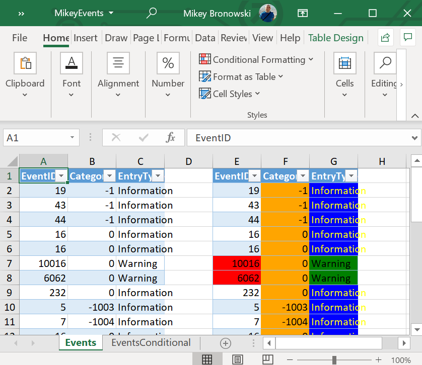
That is right. We have changed background for all the ‘warning’ values.

Finally, there is one interesting formatting using icon sets. The ImportExcel module can do it too:

# define conditional format for the IconSet using Quarters
$ConditionalFormat3 =$(
    New-ConditionalFormattingIconSet -Range A2:A6 -ConditionalFormat FiveIconSet -IconType Quarters
)
# add a new table
"L",1,2,3,4,5 | Export-Excel -WorksheetName EventsIcons -TableName EventsConditional3 -Path $excelFile -ConditionalFormat $ConditionalFormat3 -Show -Activate -KillExcel

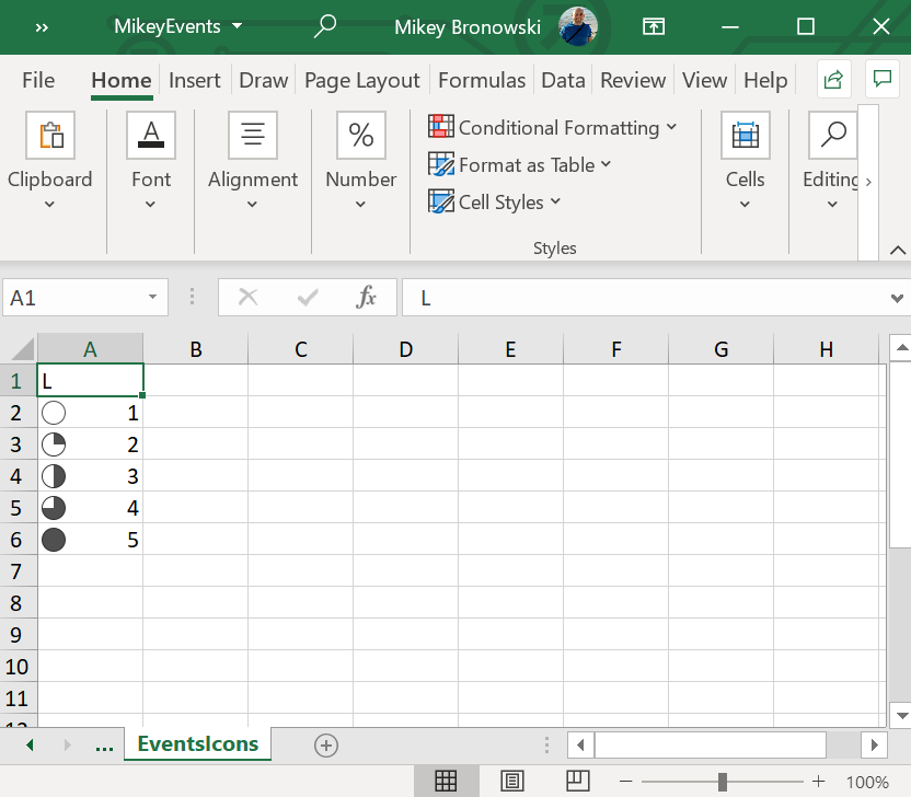
All the quarters are there! I will stop playing with the conditional formatting at this point. If you have other examples or scenarios, please comment below.

ImportExcel – how to create charts?

Last week we’ve seen how to add pivot charts, but ImportExcel module can work with regular charts as well.

As an example, I am collecting some performance counters and going to draw a chart.

# cleanup any previous files
$excelFile = "$env:TEMP\MikeyEvents.xlsx"
Remove-Item $excelFile -ErrorAction SilentlyContinue
# select your favourite counter and collect data
# this will run for 30 seconds
$counter = "\Processor(_Total)\% Processor Time"
$data = Get-Counter $counter -SampleInterval 1 -MaxSamples 30
# create a new file in TEMP location
$dataCooked = $data.CounterSamples | SELECT Path, TimeStamp, CookedValue
$chartDef = New-ExcelChartDefinition -XRange Path,TimeStamp -YRange CookedValue -ChartType Line
$dataCooked | Export-Excel -WorksheetName Events -TableName Events $excelFile -ExcelChartDefinition $chartDef -AutoNameRange -Show -KillExcel

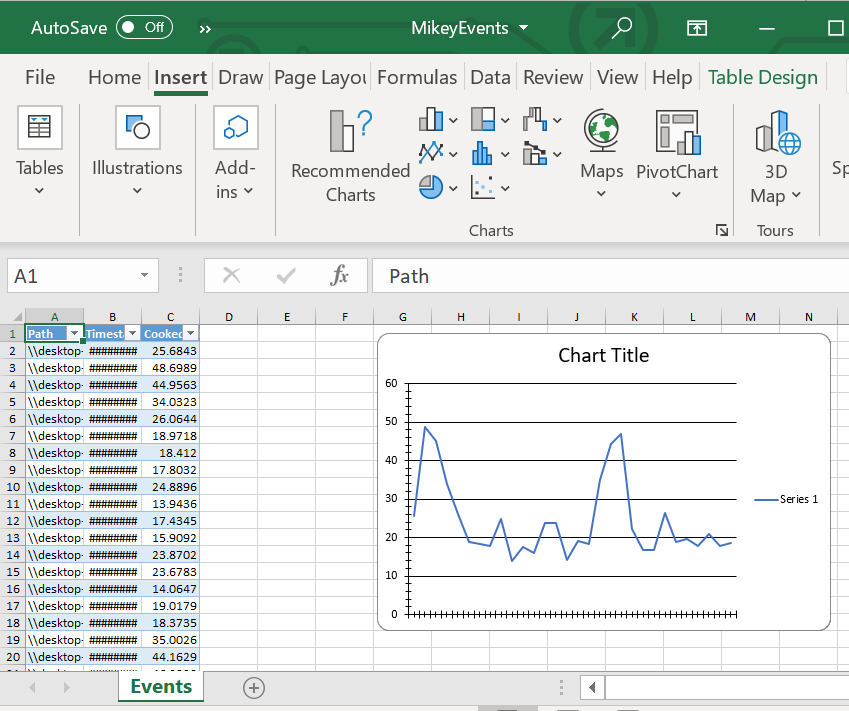
That is extremely basic chart that would need some names defined (like Title, or Series). Adding multi-series chart is also not a problem. Have a look:

# cleanup any previous files
$excelFile = "$env:TEMP\MikeyEvents.xlsx"
Remove-Item $excelFile -ErrorAction SilentlyContinue
# create an array with the data
$math = @()
for ($i=0;$i -lt 361; $i++) {
    $r = $i/180*3.14
    $math += [pscustomobject]@{ Angle = $i; Sin = [math]::Sin($r); Cos = [math]::Cos($r) }
}
# export data first
$math | Export-Excel -Path $excelFile -WorksheetName Math -AutoSize -TableName Math -KillExcel
# define the chart
$chartDef2 = New-ExcelChartDefinition -Title 'Sin(x)/Cos(x)' `
    -ChartType Line   `
    -XRange "Math[Angle]" `
    -YRange @("Math[Cos]","Math[Sin]") `
    -SeriesHeader 'Cos(x)','Sin(x)'`
    -Row 0 -Column 0
# add the chart to another worksheet
Export-Excel -Path $excelFile -WorksheetName MathChart -ExcelChartDefinition $chartDef2 -Activate -Show

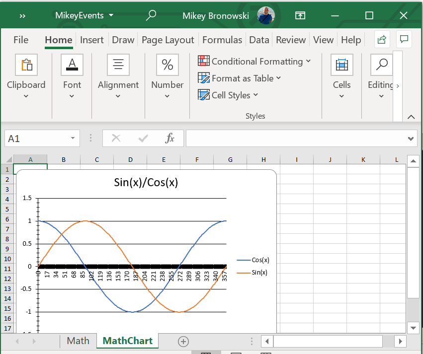The first worksheet (Math) has the data and the other one gets the beautiful sine waves.

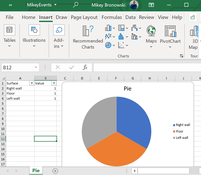
There is a way to add the chart separately, using Add-ExcelChart.

# cleanup any previous files
$excelFile = "$env:TEMP\MikeyEvents.xlsx"
Remove-Item $excelFile -ErrorAction SilentlyContinue
# define data
$data = @"
Surface,Value
Right wall,1
Floor,1
Left wall,1
"@
# export data to the excel worksheet
$data | ConvertFrom-Csv | Export-Excel -Path  $excelFile -AutoFilter -WorksheetName Pie -AutoNameRange -AutoSize -Show -KillExcel
# using Open/Close ExcelPackage add the new chart
$excel = Open-ExcelPackage $excelFile
Add-ExcelChart -Worksheet $excel.Pie -ChartType Pie -Title Pie -XRange Surface -YRange Value
Close-ExcelPackage $excel -Show

Summary

I hope you enjoyed this post and you are a bit more confident using the module. There are endless possibilities and scenarios.

Thank you,

Mikey