
How to format an entire Excel row based on the cell values with PowerShell?
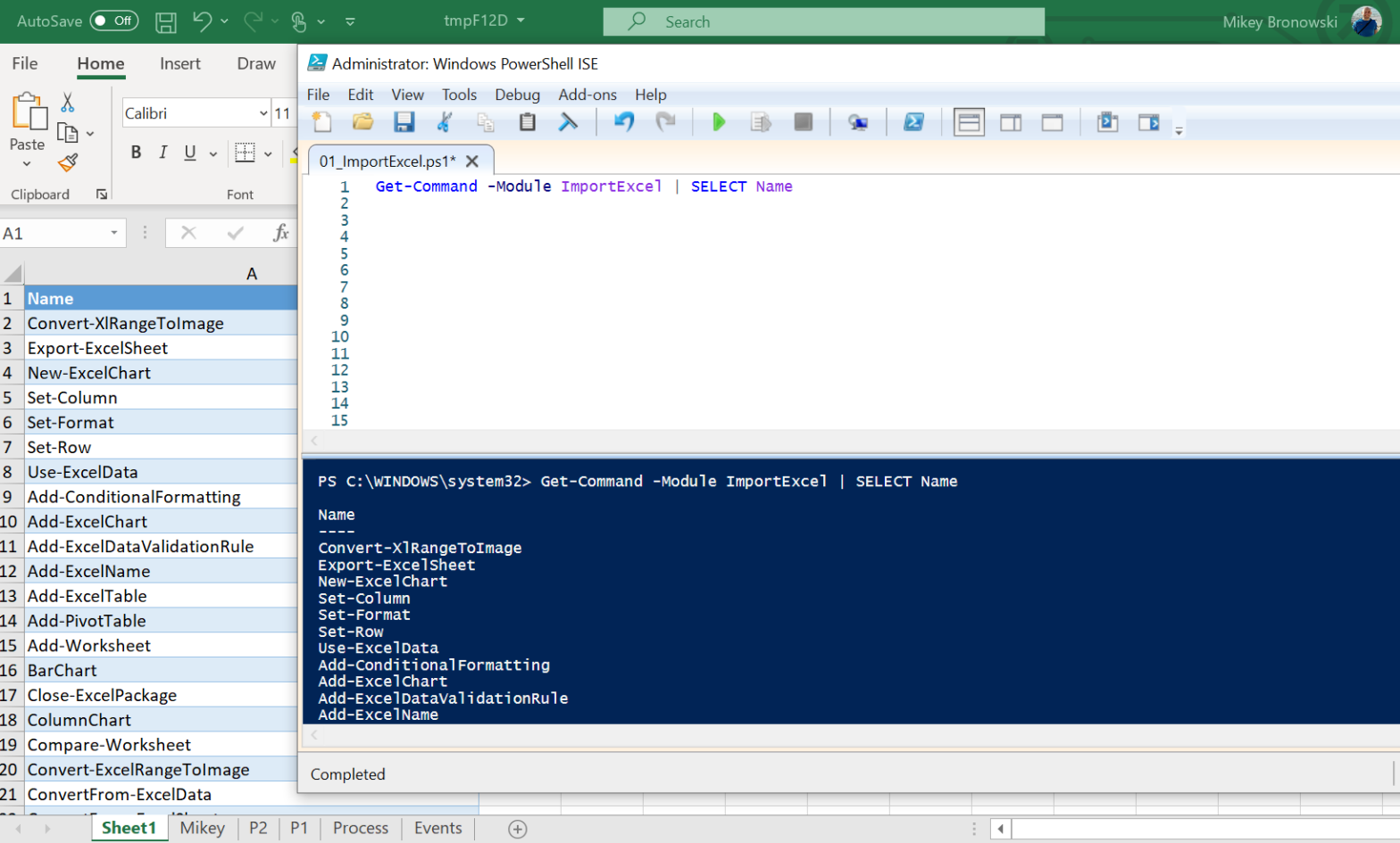
This is part of the How to Excel with PowerShell series. Links to all the tips can be found in this post. If you would like to learn more about the module with an interactive notebook, check this post out.
Another week and another tip for Excel using Powershell. Today’s post was inspired by one of my readers (thank you Harsha).
Conditional formatting is important, however by default we change the look of the cells that have specific values. What about changing the entire row if a specific cell meets certain conditions?
Preparation
Let’s prepare our environment first.
# set location for the files - I am using the temporary folder in my user profile
Set-Location $env:TEMP

# that is the location of our files
Invoke-Item $env:TEMP

# cleanup any previous files - this helps in case the example has been already ran
$excelFiles = "ImportExcelHowTo002.xlsx"
Remove-Item $excelFiles -ErrorAction SilentlyContinue
We are going to use this sample data set
# get some data
$data = ConvertFrom-Csv @'
Server,Disk,FreeSpacePct,FreeSpaceGB
SQL01,C,70,50
SQL01,D,15,200
SQL01,E,25,15
SQL01,S,55,150
SQL02,C,15,5
SQL02,D,25,300
SQL02,E,45,15
SQL02,S,65,15
SQL03,C,5,100
SQL03,D,15,10
SQL03,E,75,1
SQL03,S,15,150
'@

# pipe the data into the blank Excel file
$data | Export-Excel -Path $excelFiles -WorksheetName HowToConditionalFormatting -KillExcel -Show
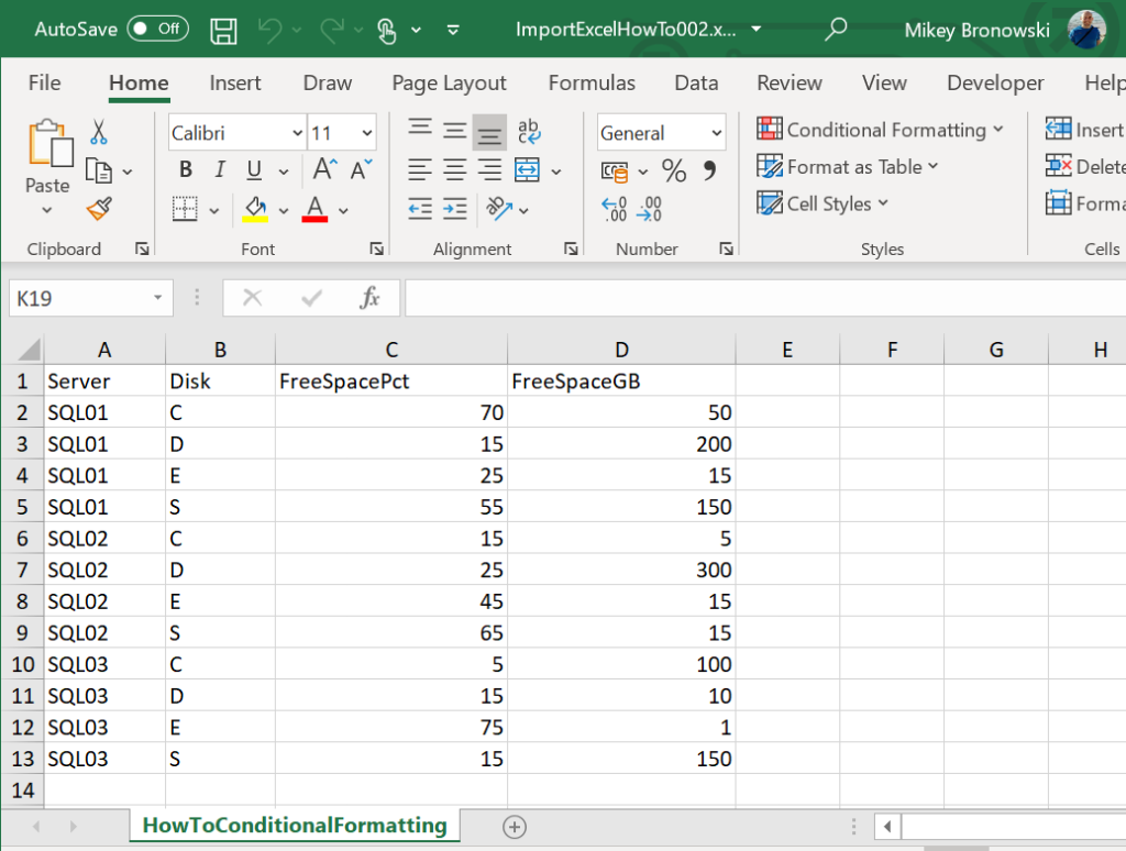
Format entire row based on the single-cell value
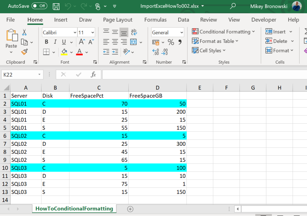
Our goal is to highlight the entire row for the C drives, so in this case rows 2, 6 and 10. To add the formatting to an existing file I am going to use a combination of Open-ExcelPackage/Add-ConditionalFormatting/Close-ExcelPackage.
For the ConditionalFormatting we want the RuleType = Expression and ConditionValue would contain our formula. Note that I am using $ sign to lock the column, so only the B column will be checked for the matching condition.
# open Excel file with PowerShell
$excelPackage = Open-ExcelPackage -Path $excelFiles -KillExcel

# get the worksheet
$excel = $excelPackage.Workbook.Worksheets['HowToConditionalFormatting']

# apply formatting to the range and put a formula in the RuleType parameter
Add-ConditionalFormatting -Worksheet $excel -Address A2:D12 -RuleType Expression -ConditionValue '=$B2="C"' -BackgroundColor Cyan

# save the changes and open the spreadsheet
Close-ExcelPackage -ExcelPackage $excelPackage -Show
And that is what we wanted to achieve:
That is neat, and we want more! What about multiple conditions?! Good question, but first…
Clean up the conditional formatting
While I was testing different things my Excel file was a collection of similar rules in the conditional formatting area. We can delete them one by one from the Excel, but there is a way to do it with PowerShell as well.
Follow the same process, open the package, do the change, close the package. In our case, I do not think there is a built-in
# open Excel file with PowerShell
$excelPackage = Open-ExcelPackage -Path $excelFiles -KillExcel

# get the worksheet
$excel = $excelPackage.Workbook.Worksheets['HowToConditionalFormatting']

# remove the conditional formatting from the whole worksheet
$excel.ConditionalFormatting.RemoveAll()

# save the changes and open the spreadsheet
Close-ExcelPackage -ExcelPackage $excelPackage -Show
That will do. The formatting is gone, so we can move on to the next step.
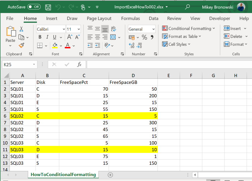
Format entire row based on the multiple cells values
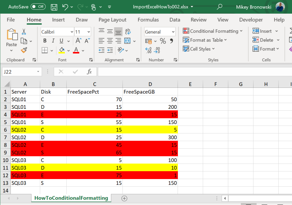
So the goal here would be here to highlight the rows where FreeSpacePct (percentage) is less than 20 and at the same time FreeSpaceGB (gigabytes) is less than 50, so rows 6 and 11.
That’s great, but how to handle multiple
Let’s add another condition to mark all the disks with FreeSpaceGB less than 20. Make them in RED.
# open Excel file with PowerShell
$excelPackage = Open-ExcelPackage -Path $excelFiles -KillExcel

# get the worksheet
$excel = $excelPackage.Workbook.Worksheets['HowToConditionalFormatting']

# apply formatting to the range and put a formula in the RuleType parameter
Add-ConditionalFormatting -Worksheet $excel -Address A2:D12 -RuleType Expression -ConditionValue '=$D2<=20' -BackgroundColor Red

# save the changes and open the spreadsheet
Close-ExcelPackage -ExcelPackage $excelPackage -Show
Rules priority
One thing to note is that every time you add the rule it gets lower priority then the existing rules, so if we switch the order of the rules added in this post the output will be different. Here is the code: cleaned up the formatting, added the RED then YELLOW (so in the reverse order):
# open Excel file with PowerShell
$excelPackage = Open-ExcelPackage -Path $excelFiles -KillExcel

# get the worksheet
$excel = $excelPackage.Workbook.Worksheets['HowToConditionalFormatting']

# remove the entire formatting
$excel.ConditionalFormatting.RemoveAll()

# apply formatting to the range and put a formula in the RuleType parameter
Add-ConditionalFormatting -Worksheet $excel -Address A2:D12 -RuleType Expression -ConditionValue '=$D2<=20' -BackgroundColor Red
Add-ConditionalFormatting -Worksheet $excel -Address A2:D12 -RuleType Expression -ConditionValue '=AND($C2<=20,$D2<=50)' -BackgroundColor Yellow

# save the changes and open the spreadsheet
Close-ExcelPackage -ExcelPackage $excelPackage -Show
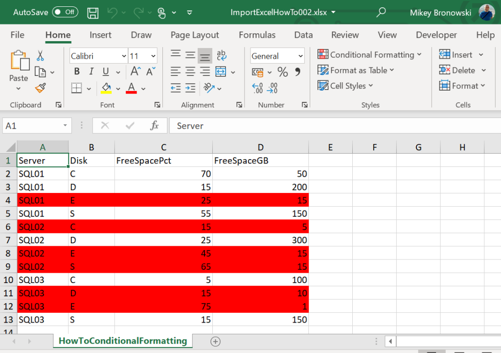
and the output does not contain any YELLOWS, because all of them were marked RED first:
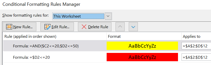
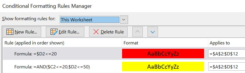
The reason is the priorities. The below image comes from YELLOW/RED example and the second one from the reverse RED/YELLOW:
We could try to change the priority of the rules as well. Try playing with the ConditionalFormatting like the example below.
# open Excel file with PowerShell
$excelPackage = Open-ExcelPackage -Path $excelFiles -KillExcel

# get the worksheet
$excel = $excelPackage.Workbook.Worksheets['HowToConditionalFormatting']

# change the priority of the first rule (Priority = 1)
$excel.ConditionalFormatting[0].Priority = 2

# save the changes and open the spreadsheet
Close-ExcelPackage -ExcelPackage $excelPackage -Show
Summary
Today I have showed you how to do the conditional formatting for the entire row based on a single or multiple cells values. We have learned how to clear up the whole conditional formatting as well as how to manage the priorities.
Thank you, Mikey